|

前言
這幾天在搞論文圖,唉說實話摳圖這種東西真能逼死人。坐在電腦前摳上一天越看越丑,最后把自己丑哭了……
到了畫折線圖分析的時候,在想用哪些工具的時候。首先否決了excel,讀書人的事,怎么能用excel畫論文的圖呢?

然后我又嘗試了Gnuplot、Matlab、Python等。這些軟件作圖無疑是一個非常好的選擇,他們都有一個共同的特點,就是圖片都是用代碼生成的。
但是學(xué)習(xí)成本太高啦。為了畫一個破圖,折騰上十天半個月,誰受得了。
像小編這種偶爾寫寫代碼日常懂點代碼的還好。但那些平時不寫代碼而且沒有代碼基礎(chǔ)又沒有一個會寫代碼的男朋友或者只有一個不會寫代碼的男朋友的女生可咋辦?

python+Matplotlib
最后挑來挑去,最終選用了python+Matplotlib。Matplotlib是著名Python的標(biāo)配畫圖包,其繪圖函數(shù)的名字基本上與 Matlab 的繪圖函數(shù)差不多。優(yōu)點是曲線精致,軟件開源免費,支持Latex公式插入,且許多時候只需要一行或幾行代碼就能搞定。
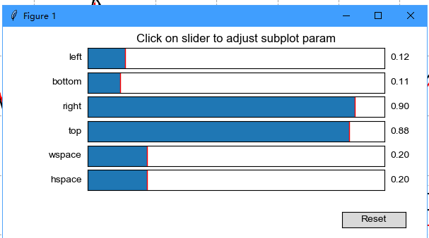
然后小編經(jīng)過了幾天的摸索,找了幾個不錯的python代碼模板,供大家簡單修改就能快速上手使用。建議使用Wing Personal 作為PythonIDE,生成的圖片能上下左右進行調(diào)整:
NO.1
# -*- coding: utf-8 -*-
import numpy as np
import matplotlib.pyplot as plt
plt.rcParams['font.sans-serif']=['Arial']#如果要顯示中文字體,則在此處設(shè)為:SimHei
plt.rcParams['axes.unicode_minus']=False#顯示負號
x = np.array([3,5,7,9,11,13,15,17,19,21])
A = np.array([0.9708, 0.6429, 1, 0.8333, 0.8841, 0.5867, 0.9352, 0.8000, 0.9359, 0.9405])
B= np.array([0.9708, 0.6558, 1, 0.8095, 0.8913, 0.5950, 0.9352, 0.8000, 0.9359, 0.9419])
C=np.array([0.9657, 0.6688, 0.9855, 0.7881, 0.8667, 0.5952, 0.9361, 0.7848, 0.9244, 0.9221])
D=np.array([0.9664, 0.6701, 0.9884, 0.7929, 0.8790, 0.6072, 0.9352, 0.7920, 0.9170, 0.9254])
#label在圖示(legend)中顯示。若為數(shù)學(xué)公式,則最好在字符串前后添加"$"符號
#color:b:blue、g:green、r:red、c:cyan、m:magenta、y:yellow、k:black、w:white、、、
#線型:- -- -. : ,
#marker:. , o v < * + 1
plt.figure(figsize=(10,5))
plt.grid(linestyle = "--") #設(shè)置背景網(wǎng)格線為虛線
ax = plt.gca()
ax.spines['top'].set_visible(False) #去掉上邊框
ax.spines['right'].set_visible(False) #去掉右邊框
plt.plot(x,A,color="black",label="A algorithm",linewidth=1.5)
plt.plot(x,B,"k--",label="B algorithm",linewidth=1.5)
plt.plot(x,C,color="red",label="C algorithm",linewidth=1.5)
plt.plot(x,D,"r--",label="D algorithm",linewidth=1.5)
group_labels=['dataset1','dataset2','dataset3','dataset4','dataset5',' dataset6','dataset7','dataset8','dataset9','dataset10'] #x軸刻度的標(biāo)識
plt.xticks(x,group_labels,fontsize=12,fontweight='bold') #默認字體大小為10
plt.yticks(fontsize=12,fontweight='bold')
plt.title("example",fontsize=12,fontweight='bold') #默認字體大小為12
plt.xlabel("Data sets",fontsize=13,fontweight='bold')
plt.ylabel("Accuracy",fontsize=13,fontweight='bold')
plt.xlim(3,21) #設(shè)置x軸的范圍
#plt.ylim(0.5,1)
#plt.legend() #顯示各曲線的圖例
plt.legend(loc=0, numpoints=1)
leg = plt.gca().get_legend()
ltext = leg.get_texts()
plt.setp(ltext, fontsize=12,fontweight='bold') #設(shè)置圖例字體的大小和粗細
plt.savefig('D:\\filename.png') #建議保存為svg格式,再用inkscape轉(zhuǎn)為矢量圖emf后插入word中
plt.show()
效果圖:
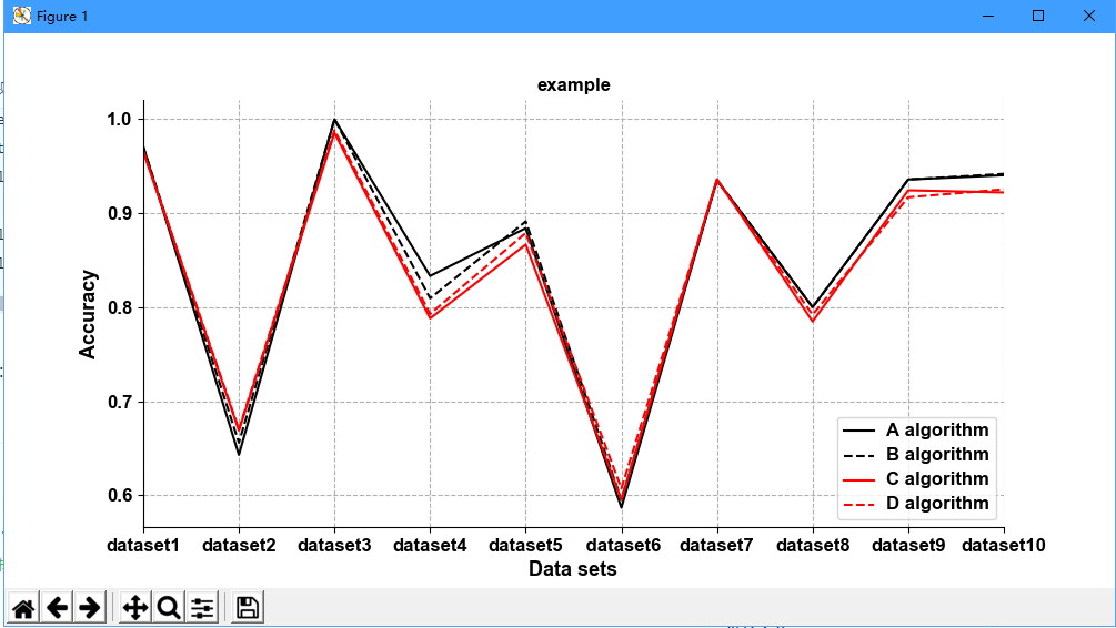
NO.2
# coding=utf-8
import numpy as np
import matplotlib.pyplot as plt
plt.rcParams['font.sans-serif'] = ['Arial'] # 如果要顯示中文字體,則在此處設(shè)為:SimHei
plt.rcParams['axes.unicode_minus'] = False # 顯示負號
x = np.array([1, 2, 3, 4, 5, 6])
VGG_supervised = np.array([2.9749694, 3.9357018, 4.7440844, 6.482254, 8.720203, 13.687582])
VGG_unsupervised = np.array([2.1044724, 2.9757383, 3.7754183, 5.686206, 8.367847, 14.144531])
ourNetwork = np.array([2.0205495, 2.6509762, 3.1876223, 4.380781, 6.004548, 9.9298])
# label在圖示(legend)中顯示。若為數(shù)學(xué)公式,則最好在字符串前后添加"$"符號
# color:b:blue、g:green、r:red、c:cyan、m:magenta、y:yellow、k:black、w:white、、、
# 線型:- -- -. : ,
# marker:. , o v < * + 1
plt.figure(figsize=(10, 5))
plt.grid(linestyle="--") # 設(shè)置背景網(wǎng)格線為虛線
ax = plt.gca()
ax.spines['top'].set_visible(False) # 去掉上邊框
ax.spines['right'].set_visible(False) # 去掉右邊框
plt.plot(x, VGG_supervised, marker='o', color="blue", label="VGG-style Supervised Network", linewidth=1.5)
plt.plot(x, VGG_unsupervised, marker='o', color="green", label="VGG-style Unsupervised Network", linewidth=1.5)
plt.plot(x, ourNetwork, marker='o', color="red", label="ShuffleNet-style Network", linewidth=1.5)
group_labels = ['Top 0-5%', 'Top 5-10%', 'Top 10-20%', 'Top 20-50%', 'Top 50-70%', ' Top 70-100%'] # x軸刻度的標(biāo)識
plt.xticks(x, group_labels, fontsize=12, fontweight='bold') # 默認字體大小為10
plt.yticks(fontsize=12, fontweight='bold')
# plt.title("example", fontsize=12, fontweight='bold') # 默認字體大小為12
plt.xlabel("Performance Percentile", fontsize=13, fontweight='bold')
plt.ylabel("4pt-Homography RMSE", fontsize=13, fontweight='bold')
plt.xlim(0.9, 6.1) # 設(shè)置x軸的范圍
plt.ylim(1.5, 16)
# plt.legend() #顯示各曲線的圖例
plt.legend(loc=0, numpoints=1)
leg = plt.gca().get_legend()
ltext = leg.get_texts()
plt.setp(ltext, fontsize=12, fontweight='bold') # 設(shè)置圖例字體的大小和粗細
plt.savefig('./filename.svg', format='svg') # 建議保存為svg格式,再用inkscape轉(zhuǎn)為矢量圖emf后插入word中
plt.show()
效果圖:
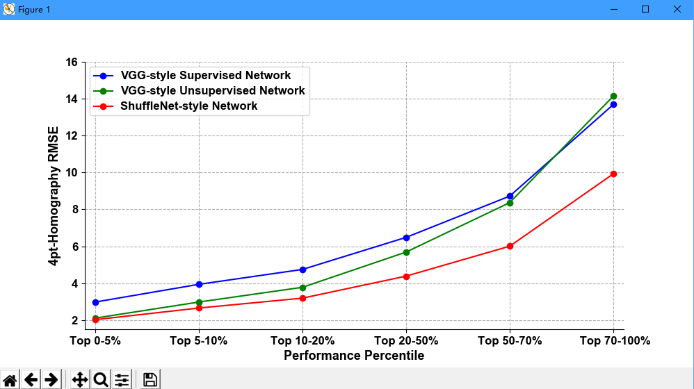
NO.3
# coding=utf-8
import matplotlib.pyplot as plt
from matplotlib.pyplot import figure
import numpy as np
figure(num=None, figsize=(2.8, 1.7), dpi=300)
#figsize的2.8和1.7指的是英寸,dpi指定圖片分辨率。那么圖片就是(2.8*300)*(1.7*300)像素大小
test_mean_1000S_n = [0.7,0.5,0.3,0.8,0.7,0.5,0.3,0.8,0.7,0.5,0.3,0.8,0.7,0.5,0.3,0.8,0.7,0.5,0.3,0.8]
test_mean_1000S = [0.9,0.8,0.7,0.6,0.9,0.8,0.7,0.6,0.9,0.8,0.7,0.6,0.9,0.8,0.7,0.6,0.9,0.8,0.7,0.6]
plt.plot(test_mean_1000S_n, 'royalblue', label='without threshold')
plt.plot(test_mean_1000S, 'darkorange', label='with threshold')
#畫圖,并指定顏色
plt.xticks(fontproperties = 'Times New Roman', fontsize=8)
plt.yticks(np.arange(0, 1.1, 0.2), fontproperties = 'Times New Roman', fontsize=8)
#指定橫縱坐標(biāo)的字體以及字體大小,記住是fontsize不是size。yticks上我還用numpy指定了坐標(biāo)軸的變化范圍。
plt.legend(loc='lower right', prop={'family':'Times New Roman', 'size':8})
#圖上的legend,記住字體是要用prop以字典形式設(shè)置的,而且字的大小是size不是fontsize,這個容易和xticks的命令弄混
plt.title('1000 samples', fontdict={'family' : 'Times New Roman', 'size':8})
#指定圖上標(biāo)題的字體及大小
plt.xlabel('iterations', fontdict={'family' : 'Times New Roman', 'size':8})
plt.ylabel('accuracy', fontdict={'family' : 'Times New Roman', 'size':8})
#指定橫縱坐標(biāo)描述的字體及大小
plt.savefig('./where-you-want-to-save.png', dpi=300, bbox_inches="tight")
#保存文件,dpi指定保存文件的分辨率
#bbox_inches="tight" 可以保存圖上所有的信息,不會出現(xiàn)橫縱坐標(biāo)軸的描述存掉了的情況
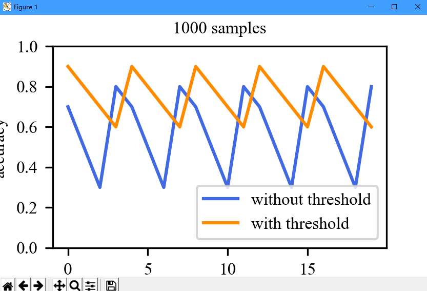
plt.show()
#記住,如果你要show()的話,一定要先savefig,再show。如果你先show了,存出來的就是一張白紙。
效果圖:
最后在放點Matplotlib相關(guān)設(shè)置供大家參考:
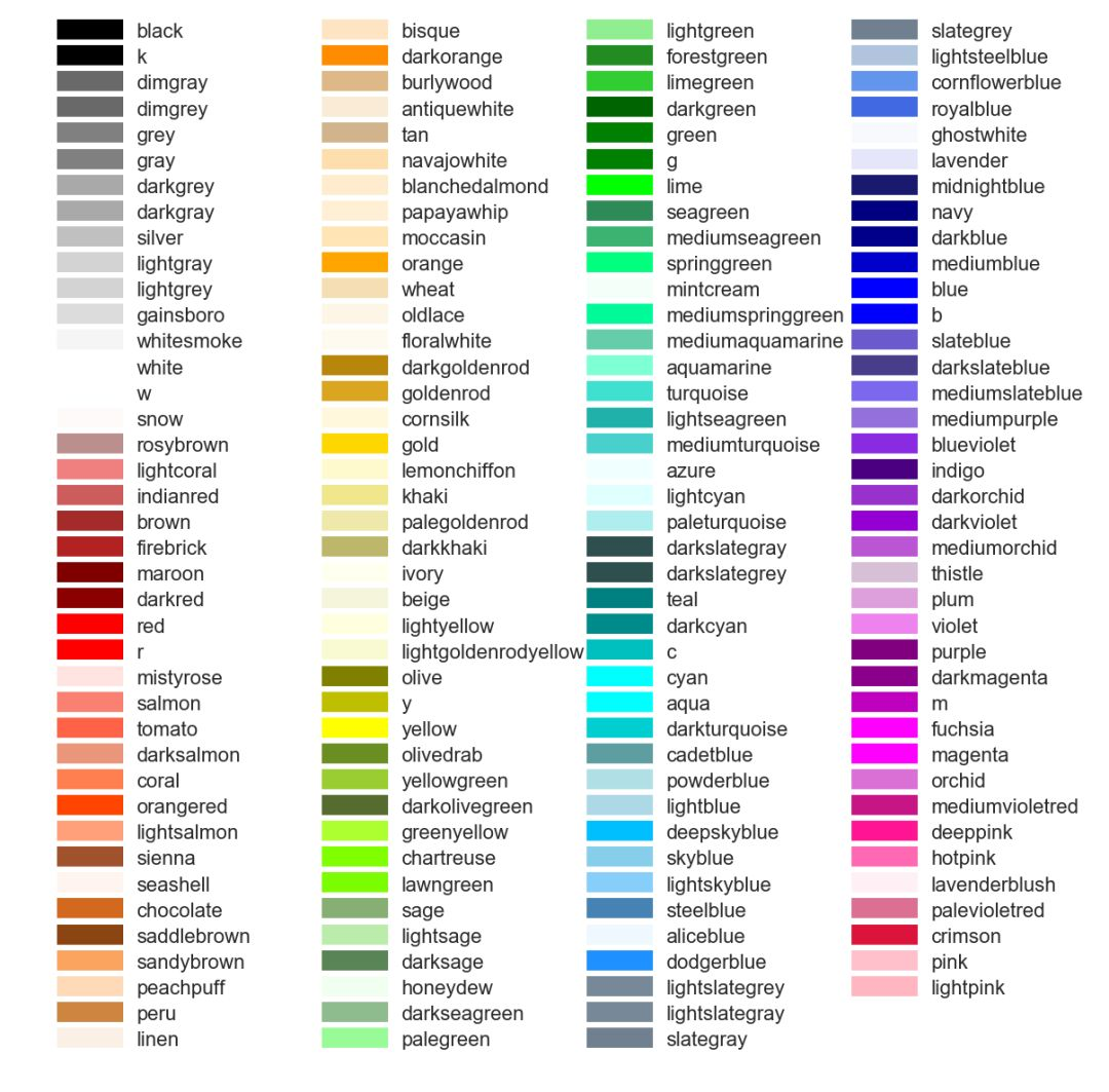
附顏色表
Marker常見參數(shù)
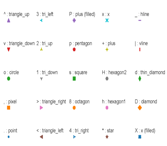
注:大家可以mark一下,說不定以后用得上呢?

最后,我還是用回了excel作圖。。。

|