| Magnetoacoustic Tomography with Magnetic Induction (MAT | 您所在的位置:網(wǎng)站首頁 › 屬蛇的男孩和屬蛇的女孩結(jié)(jié)婚好嗎婚姻如何 › Magnetoacoustic Tomography with Magnetic Induction (MAT |
Magnetoacoustic Tomography with Magnetic Induction (MAT
|
Abstract
We report our theoretical and experimental investigations on a new imaging modality, magnetoacoustic tomography with magnetic induction (MAT-MI). In MAT-MI, the sample is located in a static magnetic field and a time-varying (μs ) magnetic field. The time-varying magnetic field induces eddy current in the sample. Consequently, the sample will emit ultrasonic waves by the Lorentz force. The ultrasonic signals are collected around the object to reconstruct images related with the electrical impedance distribution in the sample. MAT-MI combines the good contrast of electrical impedance tomography with the good spatial resolution of sonography. In principle, MAT-MI mainly has two unique features due to the solenoid nature of the induced electrical field. Firstly, MAT-MI could provide explicit or simple quantitative reconstruction algorithm for the electrical impedance distribution. Secondly, it promises to eliminate the shielding effects of other imaging modalities in which the current is applied directly with electrodes. In the theoretical part, we provide the formulas for both the forward and inverse problems of MAT-MI and estimate the signal amplitude in biological tissues. In the experimental part, the experiment setup and methods are introduced and the signals and the image of a metal object by means of MAT-MI are presented. The promising pilot experimental results suggest the feasibility of the proposed MAT-MI approach. INTRODUCTIONElectrical impedance tomography (EIT) (Krestel 1990, Webb 1992, Paulson et al 1993, Morucci and Rigaud 1996) has been used in various clinical applications and continues to attract substantial research interest because of its functional information. However, the spatial resolution of EIT is low. In order to provide high spatial resolution of impedance information, we have developed a new approach called magnetoacoustic tomography with magnetic induction (MAT-MI) by combining ultrasound and magnetism. In this method, the sample is put in a static magnetic field and a time-varying (μs ) magnetic field (Fig. 1). The time-varying magnetic field induces eddy current in the sample. Consequently, the sample will emit ultrasonic waves through the Lorentz force produced by the combination of the eddy current and the static magnetic field. The ultrasonic waves are then collected by the detectors located around the sample for image reconstruction. MAT-MI combines the good contrast of EIT with the good spatial resolution of ultrasound. Fig. 1.
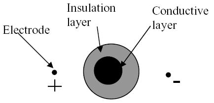
Illustration of MAT-MI. The MAT-MI is similar to magnetoacoustic tomography (MAT) (Towe and Islam 1988, Islam and Towe 1988, Roth et al 1994, Roth et al 1998) or the reverse mode of Hall effect imaging (HEI) (Wen et al 1998, Wen 1999, Wen 2000) where electric stimulation instead of magnetic stimulation is employed. In MAT and HEI/MAT the current is either spontaneous or injected into a sample by applying electrodes on the surface of the sample. As a contrast, in MAT-MI a magnetic inductor is used to generate a time-varying magnetic field, which in turn induces a pulsed electrical field and eddy current. The magnetic inductor used in MAT-MI is similar to the magnetic stimulator (MS) widely used in the research and clinical environment, especially for the intracranial delivery of magnetic energy into the brain (Irwin et al 1970, Barker et al 1990, Roth and Basser 1990 , Malmivuo and Plonsey 1995, Davey and Epstein 2000, Wagner et al 2004). But the induced electric pulse width (in the μs scale ) in the MAT-MI is much shorter than that of commercial magnetic stimulators (in the ms scale) in order to obtain the spatial resolution of mm scale. This is because the resolution in MAT-MI is approximately the electric pulse width times the acoustic speed in soft tissues (about 1.5 km/s). Compared with the other similar imaging modalities aimed at obtaining the electrical impedance distribution such as EIT, magnetic induction tomography (MIT) (Al-Zeibak et al 1995, Griffiths et al 1996, Merwa et al 2005), HEI/MAT, and magnetic resonance electrical impedance tomography (MREIT) (Woo et al 1994, Kwon et al 2002, Gao et al 2005), MAT-MI has several unique features. Firstly, it will not be affected by the low-conductivity layer of tissue at/near the surface of human body, such as the skull of the head and the fat layer of the breast. This is because the magnetic fields, unlike electrical currents, can go into the low-conductivity layer easily. For example, assume we have a two-layered object in a conductive medium (Fig. 2). The outer layer has a low conductivity like the skull or fat, while the inner layer has a high conductivity like the muscle or brain tissue. If we inject currents into the medium with electrodes, as used in EIT, HEI/MAT, and MREIT (Woo et al 1994, Kwon et al 2002, Gao et al 2005) the outer layer will reduce the amount of current entering into the inner layer. This will decrease the sensitivity to the changes of conductivity in the inner layer. As an extreme example, there will be no current in the inner layer if the outer layer is insulating. Under such extreme case, the conductivity distribution within the inner layer can not be reconstructed no matter what kind of reconstruction algorithm is used in the imaging modalities. We call this shielding effect (Wen 1999, Tidswell et al 2001). As a contrast, there is still current in the inner layer in MAT-MI even the outer layer is insulating. There is also no shielding effect in MIT due to the use of magnetic induction. But no high-spatial-resolution MIT has been reported. The second unique feature of MAT-MI is that the electrical field induced by a time-varying magnetic field in MAT-MI is a solenoid field, while irrotational fields are used in most other tomography related with the electrical properties, such as EIT, HEI/MAT, and MREIT. We find that there are explicit formulas to reconstruct conductivity from acoustic signals in MAT-MI due to this unique feature of solenoid field, as will be shown in the reconstruction methods. At last, MAT-MI is compatible with MRI setup. In both imaging modalities, the sample is located in a static magnetic field and a time-varying magnetic field. However, MAT-MI is much less demanding in the field homogeneity and stability than MRI. Fig. 2.
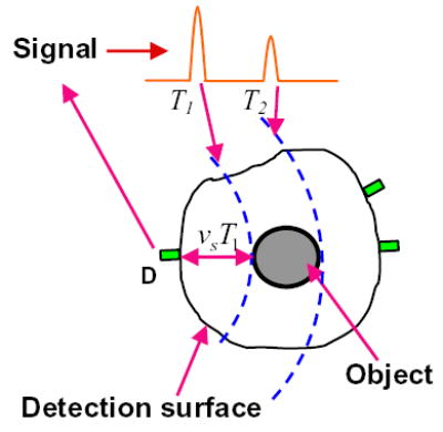
Shielding effect when injecting current with electrodes. In the Theory section, we present the formulas for both the forward and inverse problem in MAT-MI and estimate the pressure induced in biological tissues. In the Experiments section, the experimental setup and methods are introduced. The MAT-MI signals and an image from metal samples are also shown. THEORYIn this section, we first derive the formulas for the forward problem, which express the acoustic pressure in terms of the eddy current and the static magnetic field. Then, we estimate the pressure induced in biological tissue by computing the acoustic waves from a sphere in a uniform electrical and magnetic field. At last, we will provide the formulas for the inverse problem in MAT-MI. Forward problemIn a medium with a current distribution J~ (in this paper, the tilt over a variable means that the variable is a function of time; otherwise, the variable is not a function of time if not denoted explicitly) in a static magnetic field B0, we have the following wave equation for the induced pressure p~(r,t) (Roth et al 1994), ?2p~-1cs2?2p~?t2=??(J~×B0), (1)where cs=1ρ0βs is the acoustic speed, ρ0 is the density of the medium at rest, and βs is the adiabatic compressibility of the medium. We have assumed that B~1(r,t)?B0(r) in the above equation, where B~1(r,t)=B1(r)step(t) is the time-varying magnetic field in our experiments and step(t) is the step function (it equals 1 when t is larger than zero and equals zero otherwise). This is because the time-varying magnetic field is generated by discharging a capacitor for only about 1 microsecond and the current in the coil is approximately proportional to the discharging time. Therefore the current in the coil should not be large enough to produce a magnetic field that is comparable with the static magnetic field. The estimate from our experiments also supports this assumption, as will be shown in the experimental setup section. J~ in the source term can further be written as the product of a purely spatial and a purely temporal component i.e., J~(r,t)=J(r)η(t), where J(r) describes the spatial distribution of the induced eddy current density, and η(t) describes the shape of the stimulating pulse. Note that J(r) has the unit of As/m2. Here we consider J(r) to be the induced eddy current since the current generated by excitable membranes within a biological system is in the frequency of several KHz while the induced current in MAT-MI used for image reconstruction is in a much higher frequency range. We consider only the case that the stimulating pulse is very short η(t) ≈ δ(t). In experiments, the temporal profile of the induced current includes a strong short positive peak (μs) and a small long negative tail (ms). The net area under the profile is zero. But if we measure only the part of the signal that is within a short time after the positive peak (for example 100 μs ), the net area under this portion of profile is positive and we can approximate this profile as a delta function. In the following estimate on the pressure, we have J(r)≈J~ave(r)τ by using J(r)=∫0+∞J~(r,t)dt, where τ is the excitation pulse length and Jave (r) is the average current density during the excitation. After using Green’s function, the solution of Eq. 1 can be written as (Morse and Feshbach 1953) p~(r,t)=-14π∮Vdr′?r′?[J(r′)×B0(r′)]δ(t-R/cs)R, (2)where R=?|r-r′| and the integration is over the sample volume. The physical meaning of this equation is that, in an acoustically homogenous medium, the pressure p, at a spatial point r and time t, is proportional to the integration of ? · (J × B0) over a spherical surface [a circle in the two-dimensional (2-D) case]. The spherical surface is centered at r and has a radius of tcs. Applying integration by parts to Eq. 2, we have p~(r,t)=-14π∮Vdr′J(r′)×B0(r′)??r′δ(t-R/cs)R. (3)Using ?r′, = ??r, we have p~(r,t)=--14π∮Vdr′J(r′)×B0(r′)??rδ(t-R/cs)R. (4)Now the differentiation over r can be moved out of the integration and we have p~(r,t)=-14π??∮Vdr′J(r′)×B0(r′)δ(t-R/cs)R. (5)This equation is easier to compute in the theoretical analysis and numerical simulations. Estimation of the pressureWe use a spherical sample to estimate the amplitude of the MAT-MI signal from biological tissues. Assume a sphere with a radius a in a static magnetic field B0 and a time-varying magnetic field. For simplicity, we assume that B0=B0y^ and the electric field induced by the time-varying magnetic field Eext=E0x^ are homogeneous. Although the total electric field in the sphere is different from Eext (see Eq. 9), we will use Eext to approximate the total electric field for simplicity because we only want to estimate the order of the induced pressure. The sphere and background is acoustically homogeneous and has the same acoustic properties. Take the center of the sphere as the origin, the electrical conductivity of the system is σ(r)=σ0sa(r),sa(r)={1,?if?r?a.In the estimation, we use J~=σE~, where we have ignored the displacement current -?D~/?t, because the ratio of displacement to conduction current is on the scale of ω?/σ (Wang and Eisenberg 1994), where ? is the permittivity of the sample (~10?9 F/m in biological tissue) and ω is the frequency, and the ratio is on the scale of 0.001 at the MHz range in the biological tissues. The pressure can be computed through Eq. 5 as p~(r,t)=acsτσ0E0B02rz^?r^(h(t^)+h1(t^)ar). (6)where r^ is a unit vector along r , t^=(tcs-r)/a, h(t^)={-t^,?if?|t^|?1, (7)and h1(t)=∫-∞tdth(t) h1(t)={(1-t2)/2,?if?|t|?1. (8)From Eq. 6, the amplitude of the pressure can be estimated as p~(r,t)=acsτσ0E0B02r?z^?r^. We use the following parameters for estimation. a = 10mm, r = 50mm, cs = 1500m / s , τ = 0.5μs . B0 = 1T is in the same scale of commercial MRI scanners. σ = 0.2Sm?1 is typical for soft biological tissues. Eo = 1000Vm?1 is in the same scale of commercial magnetic stimulators. According to Eq. 6, we have p(r,t)=0.015?z^?r^ Pascal, which means that the pressure is anisotropic in the spatial distribution. When measuring from along z axis (which is the direction of J × B0), the amplitude is maximal, 0.015 Pa. This level of pressure should be measurable for current acoustic detectors. Inverse problemThe inverse problem can be divided into two steps. In the first step, we will reconstruct ? · (J × B0) from pressure. In the second step, we will reconstruct the conductivity distribution from ? · (J × B0). The first step can be accomplished with back-projection algorithm. The reconstruction step from ? · (J × B0) to σ is more challenging. The total electrical field in the sample can be divided into two parts E=Eext+Ersp, (9)where the first part Eext represents the solenoid electrical field induced directly by the changing magnetic field, and Ersp represents the electrical field caused by the conductivity heterogeneity of the sample (Malmivuo and Plonsey 1995). It is of electrostatic nature, so it can be expressed as the gradient of a scalar potential Ersp=-?φ. (10)Eext can be computed easily when the coil configuration is known. However, Ersp can not be measured from experiments. The challenge in the reconstruction step from ? · (J × B0) to σ lie in how to derive σ without using Ersp . From p~ to ? · (J × B0) Assume we can measure the acoustic signals across a surface ∑ around the to-be-imaged object. Let’s consider Eq. 1 for the case of J^(r,t)=J(r)δ(t). After integrating both sides of Eq. 1 over the time range (?∞,0+) , where 0+ is an infinitely small real, we have -1cs2?p~?t|t=0+=??(J×B0). (11)The spatial derivative term disappears in the integration because the pressure is zero before time zero. In the appendix, we show that Eq. 11 is still valid in an acoustically heterogeneous medium. Eq. 11 means that we can obtain ? · (J × B0) if we can derive -1cs2?p~?t|t=0+from the pressure measured over ∑. In an acoustically homogeneous medium, this step can be accomplished by time reversing the acoustic waves using Eq. 15 in (Xu and Wang 2004a) as p~′(r,0+)≈12πcs∫Σ∫dSdn?(rd-r)|r-rd|2p~″(rd,|r-rd|/cs), (12)where rd is a point on the detection surface ∑, r is a point in the object space, and the single and double prime represent the first and second derivative over time, respectively. In deriving Eq. 12, we have ignored the first term in the integrand on the right hand side of Eq. 15 in (Xu and Wang 2004a), because it is much smaller than the second term in the MHz range. Combining Eq. 11 and Eq. 12, we have ??(J×B0)≈-12πcs3∫Σ∫dSdn?(rd-r)|r-rd|2p~″(rd,|r-rd|/cs) (13)This is a back-projection algorithm, in which the pressure at each time point is projected (assigned) to each point on the sphere over which the integration of the object value yields the pressure, as shown in Fig. 3. Fig. 3.
Illustration of backprojection. From ? · (J × B0) to σ Here we propose two methods for the second step in the reconstruction. Method 1 Piecewise distributionIn this method, we don’t need to change the direction of the static magnetic field B0 because only one set of measurement is needed. This is a major advantage of this method over the other methods. First, according to Faraday’s law, ?×E~=-?B~1?t. (14)Using B~1(r,t)=B1(r)step(t), we have E~(r,t)=E(r)δ(t), where E is the spatial component of the electrical field and obeys ?×E=-B1. (15)Combing Eq. 15 with J = σE , we have ?×(J/σ)=-B1. (16)After expanding the cross product, we have (?×J)/σ+?(1σ)×J=-B1. (17)If we assume the sample is piecewise smooth, then we have |?σ|/σ |? × J| / |J|. The result given by Eq. 18 can be improved iteratively by the following algorithm: σn=-(?×J)?B0[B1+?(1/σn-1)×Jn-1]?B0, (19)where (? × J) · B0 , B0 , and B1 are measured or derived from measurement in the experiments, σn?1 and σn are the conductivity distribution obtained after the (n?1)-th and n-th iteration, respectively, and Jn?1 is the computed current distribution corresponding to σn?1 . To start the iteration, σ0 is given by Eq. 18. Then for the given σn?1 and boundary conditions, Jn?1 can be computed by solving the forward linear system of equations using the conjugate gradient method for sparse matrix. After that, the conductivity will be updated according to Eq. 19 in each iteration until a stopping condition is met. Method 2: Solve JIn the second method, we need to change the direction of the static magnetic field B0. According to ω?/σ |

【本文地址】
| 今日新聞 |
| 推薦新聞 |
| 專題文章 |